Illustration via ChatGPT.
There are three hard things in computer science. One is making ChatGPT write “Invalidation” correctly on an image.
There’s a saying that goes: “There are only two hard things in computer science: cache invalidation and naming things.” Well, I’d argue there are actually three:
Yes, that’s a nerdy joke. No, I’m not sorry.
In this post, we’ll dive into parallel and asynchronous programming, why it matters for {shiny} developers, and how you can implement it in your next app.
Parallel vs asynchronous
The terms parallel and asynchronous are often used interchangeably when referring to “computing something elsewhere” (e.g., in another R session). However, they describe distinct approaches and require different mindsets.
Parallel
Parallel programming follows the split/apply/combine or map-reduce paradigm:
- Divide a task into
nchunks. - Compute each chunk independently (often in separate R sessions).
- Combine the results into a final output.
In R, this concept is embodied by the *apply family and its {purrr} counterpart. Here’s a simple example:
lapply(
  c("1", 12, NA),
  \(x) {
    Sys.sleep(1) # Simulate computational time
    sprintf("I'm %s", x)
  }
)
Here, each element is processed sequentially, one at a time. The tasks are independent and there is no need for communication between chunks.

This type of computational problem is “embarrassingly parallel”, i.e. it can be easily divided into independent tasks that require no communication or coordination between them. That’s why it works well in parallel : each task can be executed at the same time, with minimal effort or overhead, and no need for communication between the tasks.
In R, modern parallel processing is done via {future}, a package that provides a unified framework for parallel & distributed computation. As a framework, it comes with other packages that have implemented functions on top of it. For example the {future.apply} package, that turns the apply family into parallel processing.
Here’s how we can adapt the code:
library(future)
library(future.apply)
plan(
  strategy = multisession,
  workers = 3
)
future_lapply(
  c("1", 12, NA),
  \(x){
    # Mimicking some computational time
    Sys.sleep(1)
    sprintf("I'm %s", x)
  }
)
So, what happens here?
- First, we configured
{future}to use 3 different R sessions — schematically,{future}will open and interact with 3 different R processes on your machine. - We turn
lapplyintofuture_lapply, meaning that each\()will be run into another session, at the same time. - Then the result is combined into a list, bringing us the same result as before.
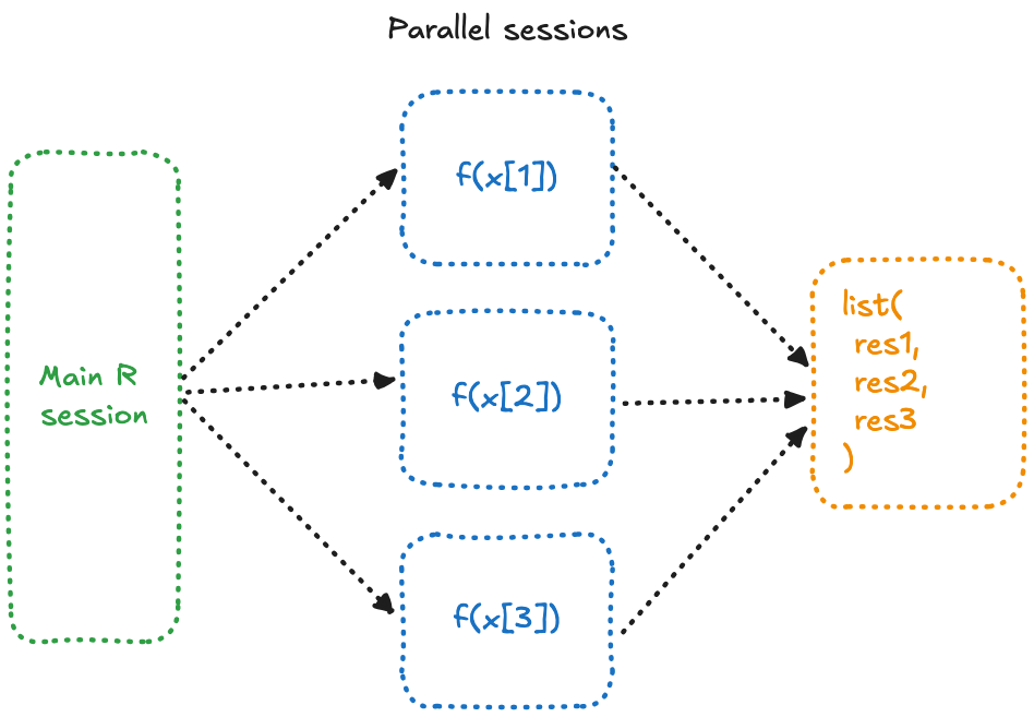
So, what’s the difference here?
Well, with the standard lapply(), the \() are executed one after the other, meaning that each iteration will take 1 second, and the whole process will take 3.
On the other hand, with future_lapply(), each \() is executed at the same time on each session, meaning that the whole computation will take 1 second (well, a bit more because you need to take into account the transportation of objects from one session to the others and back, but that’s not the point).
Let’s compare the timing of sequential and parallel execution:
system.time({
  lapply(
    c("1", 12, NA),
    \(x){
      # Mimicking some computational time
      Sys.sleep(1)
      sprintf("I'm %s", x)
    }
  )
})
   user  system elapsed
  0.001   0.001   3.017
system.time({
  future_lapply(
    c("1", 12, NA),
    \(x){
      # Mimicking some computational time
      Sys.sleep(1)
      sprintf("I'm %s", x)
    }
  )
})
   user  system elapsed
  0.090   0.007   1.205
So to sum up, parallel computing can be viewed as: “take this, cut it in small pieces, send it to other places, and I’ll wait for you to do something in those places and give it back to me”.
Drawbacks of parallel computing
More CPU/memory
More CPU and memory are consumed when running multiple R sessions, which can be a limitation if your hardware is constrained. However, as the saying goes, “you can always buy more hardware, but you can’t buy more time.”
The cost of transportation
Parallel processing is great because it can speed up tasks that would otherwise take longer to compute.
However, you need to account for the “cost of transportation.” When computations occur in a different R session, R must transfer data and load the necessary packages into that session. Here’s how this process works:
- Static Analysis: R analyzes the code to determine which data and packages are needed.
- Data Transfer: The data is written to disk and reloaded in the new session.
- Result Retrieval: The computation results are written back to disk and read into the main session.
This overhead can sometimes exceed the computational cost itself. For example, consider the following scenario:
big_m <- matrix(
  sample(1:1e5, 1e5),
  nrow = 10
)
diams <- purrr::map_df(
  rep(
    ggplot2::diamonds,
    n = 100
  ),
  identity
)
system.time({
  lapply(
    list(
      diams,
      big_m
    ),
    \(x){
      dim(x)
    }
  )
})
   user  system elapsed
  0.001   0.000   0.000
system.time({
  future_lapply(
    list(
      diams,
      big_m
    ),
    \(x){
      dim(x)
    }
  )
})
   user  system elapsed
  0.037   0.003   0.066
Think of it like this: if it takes you 20 seconds to wrap a Christmas gift, and you have three gifts to wrap, you might wonder if it’s worth outsourcing. Imagine spending 5 seconds walking the gifts to your children, 10 seconds explaining how to wrap them (which they’ll also take 20 seconds to do), and then another 5 seconds to bring them back to the table. In this case, the overhead of delegation might outweigh the benefits, and you’d be better off doing it yourself!
NERD DIGRESSION ON: ever wonder how {future} does the code analysis? Well, with the {globals} package:
expr_to_be_run <- substitute({
  lapply(
    list(
      # using shorter object for more
      # redable output
      matrix(1:2),
      1:2
    ),
    \(x){
      dim(x)
    }
  )
})
globals::globalsOf(expr_to_be_run)
$`{`
.Primitive("{")

$lapply
function (X, FUN, ...)
{
    FUN <- match.fun(FUN)
    if (!is.vector(X) || is.object(X))
        X <- as.list(X)
    .Internal(lapply(X, FUN))
}
<bytecode: 0x14e913970>
<environment: namespace:base>

$list
function (...)  .Primitive("list")

$matrix
function (data = NA, nrow = 1, ncol = 1, byrow = FALSE, dimnames = NULL)
{
    if (is.object(data) || !is.atomic(data))
        data <- as.vector(data)
    .Internal(matrix(data, nrow, ncol, byrow, dimnames, missing(nrow),
        missing(ncol)))
}
<bytecode: 0x14f283d28>
<environment: namespace:base>

$`:`
.Primitive(":")

$dim
function (x)  .Primitive("dim")

attr(,"where")
attr(,"where")$`{`
<environment: base>

attr(,"where")$lapply
<environment: base>

attr(,"where")$list
<environment: base>

attr(,"where")$matrix
<environment: base>

attr(,"where")$`:`
<environment: base>

attr(,"where")$dim
<environment: base>

attr(,"class")
[1] "Globals" "list"
NERD DIGRESSION OFF.
Asynchronous
Now, let’s explore asynchronous programming, which differs fundamentally from parallel execution.
Asynchronous programming also involves “computing elsewhere,” but the key difference is that you don’t divide a task into chunks and wait for the results to come back. Instead, the mindset with asynchronous code is: “Send this task to run elsewhere, give me back control immediately, and I’ll check in later to see if it’s done.”
This approach is precisely what future() is designed to handle:
# Reconfiguring
library(future)
plan(
  strategy = multisession,
  workers = 3
)
# Identifying current session ID
Sys.getpid()
[1] 23667
my_future <- future({
  Sys.sleep(1)
  Sys.getpid()
})
print("I immediately have my console")
"I immediately have my console" # Check if the future is resolved, i.e. if it has returned
resolved(my_future)
[1] FALSE
Sys.sleep(1)
resolved(my_future)
[1] TRUE
value(my_future)
[1] 41533
In essence, asynchronous programming involves sending a computation to be performed elsewhere without worrying about the exact moment the result will be ready. This is in contrast to parallel computing, where the timing matters because you need to gather and combine the results from all tasks.
To summarize:
- Parallel computing is blocking—you wait for all results to be ready before proceeding.
- Asynchronous computing is non-blocking—you continue working and check back for the results when they’re ready.
Managing Async Results with {promises}
Asynchronous workflows introduce two challenges:
- 1. Tracking task completion: How do you know when a task is done?
We could have something like this:
my_future <- future({ Sys.sleep(1) Sys.getpid() }) while(!resolved(my_future)){ Sys.sleep(0.1) } value(my_future)[1] 41533
But that defeats the very value of asynchronous programming, i.e. being non blocking.
- 2. Handling results: What actions should you take when the task completes successfully or fails?
A challenge with asynchronous programming is that it separates the computation from what you do with the result. You send a task off to be computed elsewhere, and when it eventually returns, you need to handle it. Ideally, there would be a way to define both the asynchronous task and its response logic together, so everything—what to compute and how to process the result—is written in one cohesive place.
future() + promise()
This is where {promise} comes into play. Inspired by how JavaScript manages asynchronous programming (or at least how it used to), {promise} provides two key features:
- It actively monitors (or polls) the
futureto check when it is resolved. - It allows you to define functions that will execute once the
futureis complete.
The default structure looks like this :
library(future)
library(promises)

fut <- future({
  Sys.sleep(3)
  1 + 1
})
then(fut,
  onFulfilled = \(result) {
    # What happens if the future resolved and returns
    cli::cat_line("Yeay")
    print(result)
  },
  onRejected = \(err) {
    # What happens if the future
    cli::cat_line("Ouch")
    print(err)
  }
)
finally(
  fut,
  \(){
    cli::cat_line("Future resolved")
  }
)
Here, we have everything in one place:
- The asynchronous code.
- What to do when it returns a value.
- What to do if it fails.
- What to do every time, regardless of success or failure.
If you run this code in your console, you’ll immediately regain control of the console. After 5 seconds, you’ll see the output as the task completes.
To make this process even smoother, the {promise} package provides wrappers that allow you to write this code in a more pipe-friendly format:
library(magrittr)
future({
  Sys.sleep(3)
  1 + 1
}) %>%
  then(\(result){
    cli::cat_line("Yeay")
    print(result)
  }) %>%
  catch(\(error){
    cli::cat_line("Ouch")
    print(err)
  }) %>%
  finally(\(){
    cli::cat_line("Future resolved")
  })
Or, even shorter:
library(magrittr)
future({
  Sys.sleep(3)
  1 + 1
}) %...>% (\(result){
    cli::cat_line("Yeay")
    print(result)
  }) %...!% (\(error){
    cli::cat_line("Ouch")
    print(err)
  }) %>%
  finally(\(){
    cli::cat_line("Future resolved")
  })
So, which approach is better? That’s entirely up to you.
Personally, I find the fully piped version more concise and elegant. However, the version with explicit function names (then, catch, etc.) makes the logic easier to follow and the code more approachable for new developers. It’s a trade-off between brevity and clarity.
Ok, but why the long post?
Async in {shiny}
If you’re still reading, you might be wondering: “Okay, but why should I care?” Let me explain why this matters if you’re a {shiny} developer.
By default, R is single-threaded, meaning it can handle only one task at a time. The same is by extension true for {shiny}: it processes one operation at a time. This means that if User A triggers a computation, User B’s action can only start once User A’s task is complete.
In most cases, this isn’t a problem—R computations are typically fast. If User B has to wait 0.1 seconds for User A’s task to finish, they likely won’t even notice.
However, this behavior becomes an issue when your app involves heavy computations, such as rendering an RMarkdown report based on app inputs. Even a small RMarkdown document can take a couple of seconds to render, which is too long in a multi-user app.
Here’s a simple example to illustrate this point:
library(shiny)

ui <- fluidPage(
  actionButton(
    inputId = "launch",
    label = "Launch Computation"
  ),
  textOutput("time"),
  textOutput("rnorm")
)

server <- function(input, output, session) {
  r <- reactiveValues()
  output$time <- renderText({
    invalidateLater(1000)
    format(Sys.time(), "%H:%M:%S")
  })
  observeEvent(input$launch, {
    Sys.sleep(3)
    r$norm <- rnorm(10)
  })
  output$rnorm <- renderText({
    r$norm
  })
}
shinyApp(ui = ui, server = server)
If you open this app in two separate browser tabs and click the button in one, you’ll notice that it freezes the app in the other. This happens because the observeEvent is blocking the entire R session while it processes the task.
But what if we applied what we learned earlier with {future}? Let’s give it a shot:
library(shiny)
library(future)
library(promises)

plan(
  strategy = multisession,
  workers = 3
)

ui <- fluidPage(
  actionButton(
    inputId = "launch",
    label = "Launch Computation"
  ),
  textOutput("time"),
  textOutput("rnorm")
)

server <- function(input, output, session) {
  r <- reactiveValues()
  output$time <- renderText({
    invalidateLater(1000)
    format(Sys.time(), "%H:%M:%S")
  })
  observeEvent(input$launch, {
    future({
      Sys.sleep(10)
      rnorm(10)
    },
    seed=TRUE
   ) %>%
      then(\(result){
        cli::cat_line("Yeay")
        r$norm <- result
      }) %>%
      catch(\(error){
        cli::cat_line("Ouch")
        r$norm <- NULL
      })
      # Render has to return otherwise it blocks
      return(NULL)
  })
  output$rnorm <- renderText({
    r$norm
  })
}
shinyApp(ui = ui, server = server)
Let’s now open this app three times, and click on the button. That works as expected. Now, let’s open 4 and click on the four in a row. Yep, everything is blocked now.
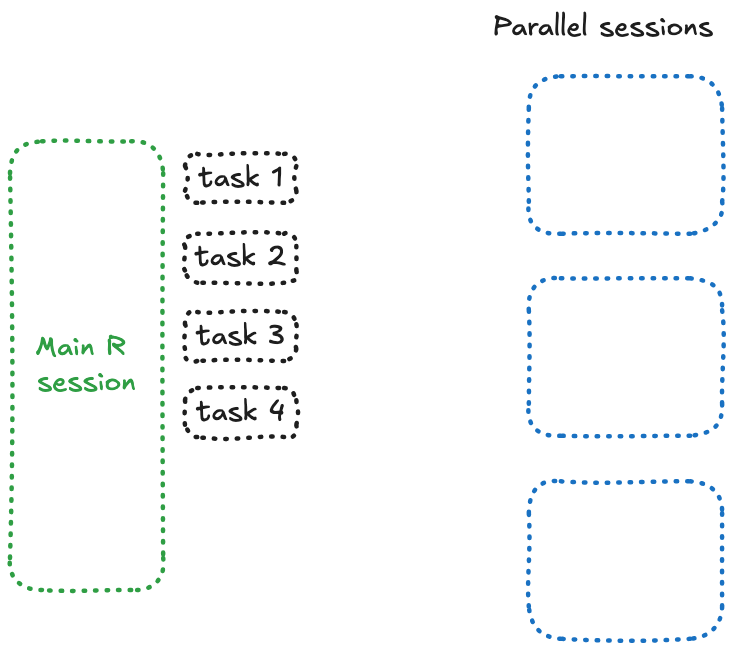
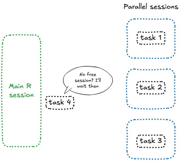
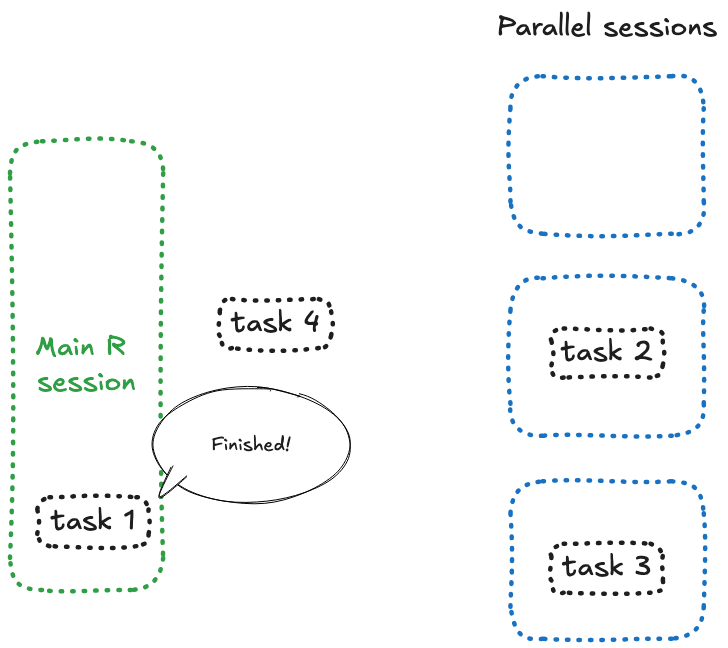
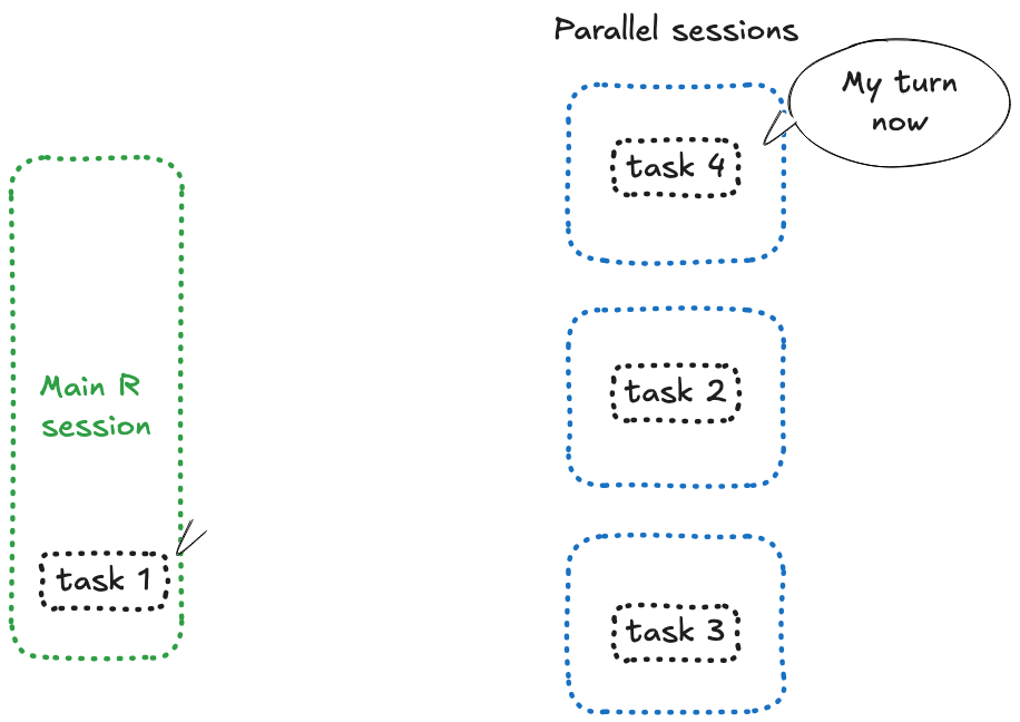
The reason is simple: something, somewhere, is blocked — and if you paid attention to the number, that’s because you’re asking to send 4 future in 3 sessions. And what happens here is that when future doesn’t have any free session, it blocks and wait.
This is something you can reproduce in a plain R session:
library(future)
plan(
  strategy = multisession,
  workers = 3
)
a <- future({
  Sys.sleep(4)
})
b <- future({
  Sys.sleep(4)
})
c <- future({
  Sys.sleep(4)
})
d <- future({
  Sys.sleep(4)
})
Something like this happens:
Woaw, that’s not good.
future_promise()
Enter future_promise(), a smarter wrapper around future() and promise() that allow to avoid the blocking issue we encountered earlier.
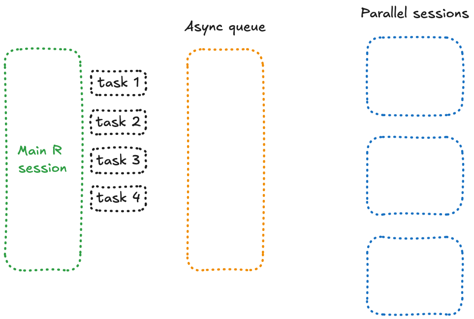
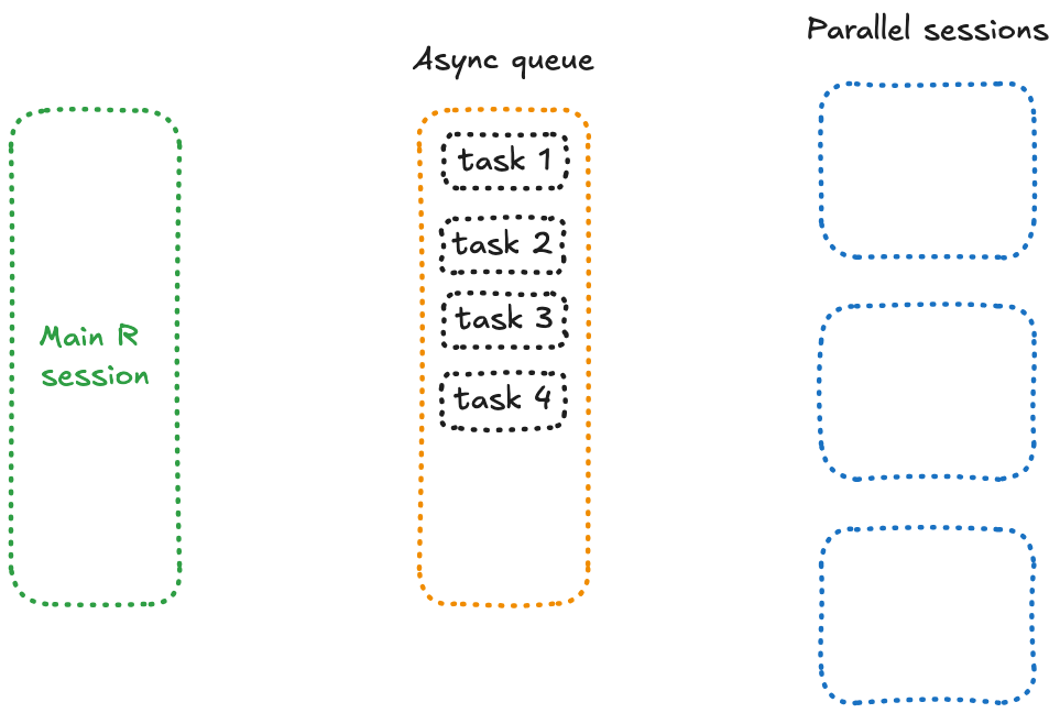
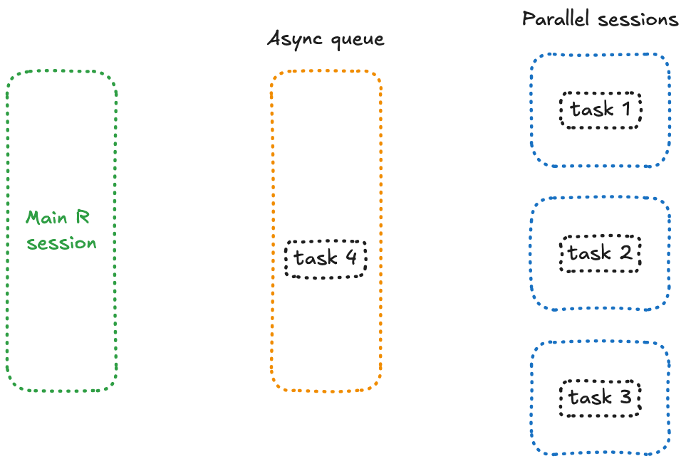
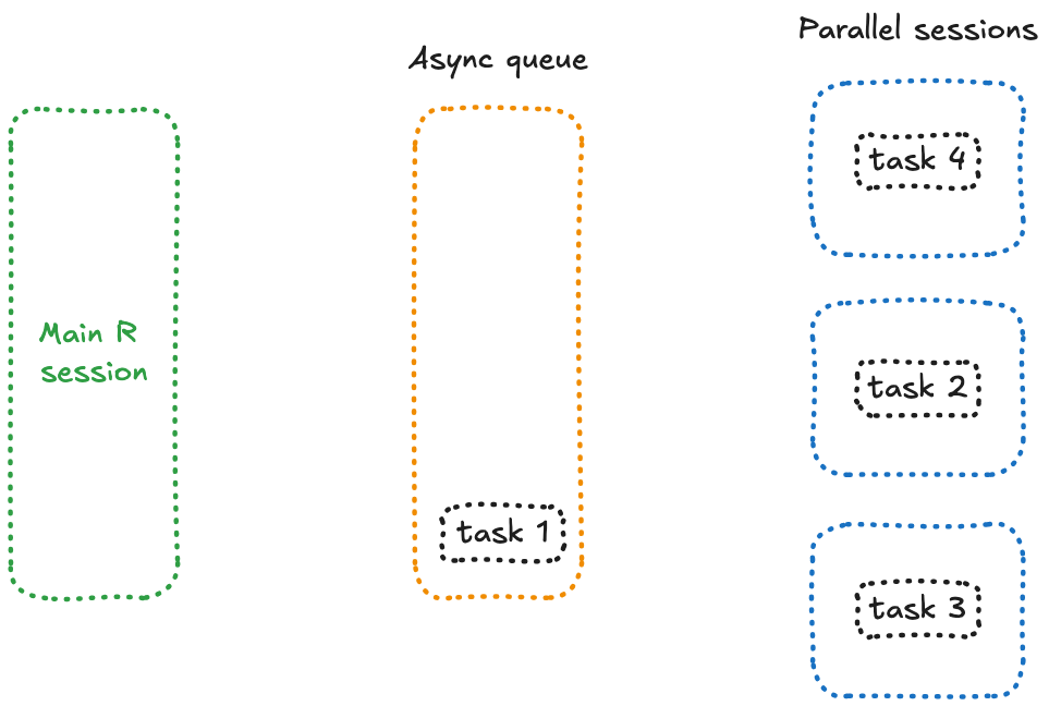
What makes future_promise() different is that it creates an asynchronous queue to manage all future() calls. Instead of blocking the main session when workers are busy, it queues up tasks and launches them as spots in the future() workers become available.
Conceptually, this means that all your pending tasks are sitting in a queue in a separate session, waiting for a free worker to process them—something like this:
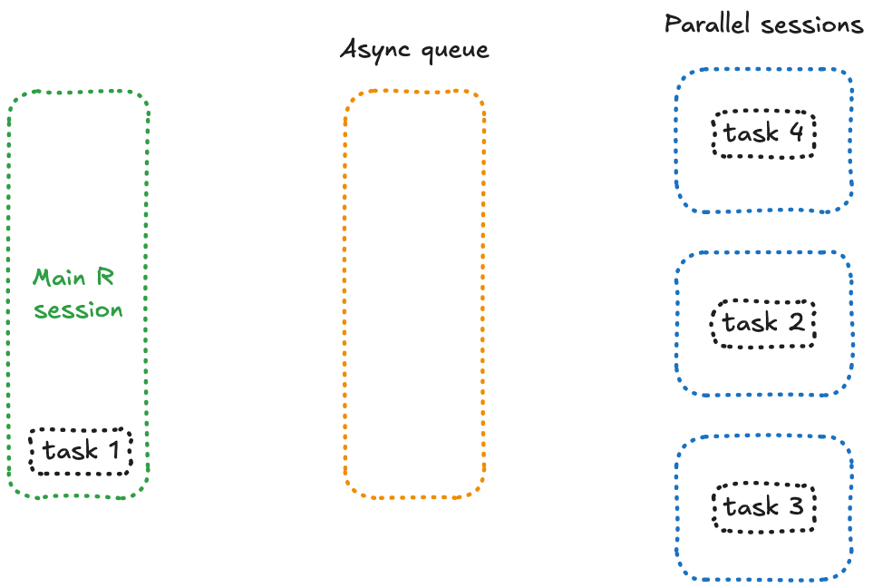
With this mechanism in place, here’s the updated version of our code:
library(shiny)
library(future)
library(promises)

plan(
  strategy = multisession,
  workers = 3
)

ui <- fluidPage(
  actionButton(
    inputId = "launch",
    label = "Launch Computation"
  ),
  textOutput("time"),
  textOutput("rnorm")
)

server <- function(input, output, session) {
  r <- reactiveValues()
  output$time <- renderText({
    invalidateLater(1000)
    format(Sys.time(), "%H:%M:%S")
  })
  observeEvent(input$launch, {
    future_promise({
      Sys.sleep(10)
      rnorm(10)
    },
    seed=TRUE
   ) %>%
      then(\(result){
        cli::cat_line("Yeay")
        r$norm <- result
      }) %>%
      catch(\(error){
        cli::cat_line("Ouch")
        r$norm <- NULL
      })
      # Render has to return otherwise it blocks
      return(NULL)
  })
  output$rnorm <- renderText({
    r$norm
  })
}
shinyApp(ui = ui, server = server)
Yeay! Now our app works as intended 🎉.
However, there’s one thing to keep in mind: since this is a queue, if you send 4 futures to 3 sessions, the 4th task will only start once the 1st task finishes (e.g., after 10 seconds). This means the total waiting time might still be significant for some tasks.
Enter the New Challenger: shiny::ExtendedTask
Implementing this with future_promise() can feel a bit complex. Fortunately, as of version 1.8.1, {shiny} includes native asynchronous support via the ExtendedTask R6 class. This class provides built-in reactive behavior for managing async tasks seamlessly.
Let’s rework our previous example using ExtendedTask:
library(shiny)
library(future)
library(promises)

plan(
  strategy = multisession,
  workers = 3
)

ui <- fluidPage(
  actionButton(
    inputId = "launch",
    label = "Launch Computation"
  ),
  textOutput("time"),
  textOutput("rnorm")
)

server <- function(input, output, session) {
  et_r_norm <- ExtendedTask$new(function() {
    future_promise({
      Sys.sleep(3)
      rnorm(10)
    }, seed = TRUE)
  })
  output$time <- renderText({
    invalidateLater(1000)
    format(Sys.time(), "%H:%M:%S")
  })
  observeEvent(input$launch, {
    et_r_norm$invoke()
  })
  output$rnorm <- renderText({
    et_r_norm$result()
  })
}
shinyApp(ui = ui, server = server)
Of course, it can take inputs from the shiny app:
library(shiny)
library(future)
library(promises)

plan(
  strategy = multisession,
  workers = 3
)

ui <- fluidPage(
  input_task_button(
    id = "launch",
    label = "Launch Computation"
  ),
  numericInput(
    "rnorm_size",
    "How many rnorm?",
    value = 10,
    min = 1,
     max = 10
  ),
  textOutput("time"),
  textOutput("rnorm")
)

server <- function(input, output, session) {
  et_r_norm <- ExtendedTask$new(function(r_norm_n) {
    future_promise({
      Sys.sleep(3)
      rnorm(r_norm_n)
    }, seed = TRUE)
  })
  output$time <- renderText({
    invalidateLater(1000)
    format(Sys.time(), "%H:%M:%S")
  })
  observeEvent(input$launch, {
    et_r_norm$invoke(input$rnorm_size)
  })
  output$rnorm <- renderText({
    et_r_norm$result()
  })
}
shinyApp(ui = ui, server = server)
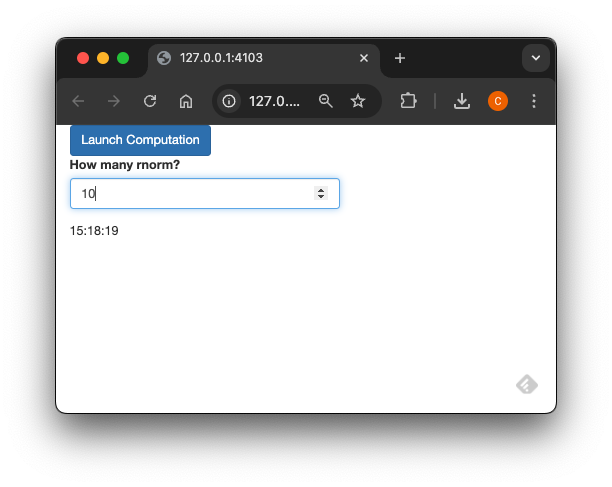
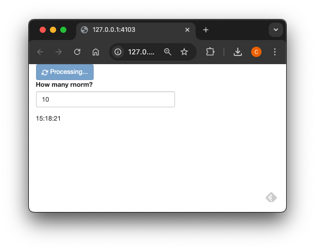
We can enhance the user experience by adding a button from {bslib} that displays a loading indicator while the task is running. This provides visual feedback to users, letting them know their request is being processed. Here’s how to integrate it:
library(shiny)
library(bslib)
library(future)
library(promises)

plan(
  strategy = multisession,
  workers = 3
)

ui <- fluidPage(
  input_task_button(
    id = "launch",
    label = "Launch Computation"
  ),
  numericInput(
    "rnorm_size",
    "How many rnorm?",
    value = 10,
    min = 1,
     max = 10
  ),
  textOutput("time"),
  textOutput("rnorm")
)

server <- function(input, output, session) {

  et_r_norm <- ExtendedTask$new(function(r_norm_n) {
    future_promise({
      Sys.sleep(3)
      rnorm(r_norm_n)
    }, seed = TRUE)
  })|> bind_task_button("launch")

  output$time <- renderText({
    invalidateLater(1000)
    format(Sys.time(), "%H:%M:%S")
  })

  observeEvent(input$launch, {
    et_r_norm$invoke(input$rnorm_size)
  })

  output$rnorm <- renderText({
    et_r_norm$result()
  })

}
shinyApp(ui = ui, server = server)
Final Words
We’ve explored how parallel and asynchronous programming represent two distinct mindsets and approaches, even though they can be combined—for instance, an asynchronous task can trigger parallel computations.
Mastering these techniques can significantly enhance the user experience of your apps, especially when dealing with long-running tasks or high user traffic.
Still unsure how to implement these concepts in your app? Tried it but things aren’t working as expected? Let’s chat!


