Interact with PostGIS from R

PostGIS extends capabilities of PostgreSQL database to deal with spatial data. Using PostGIS, your database supports geographic queries to be run directly in SQL. In this blog post, we will connect and interact with a PostGIS database from R, using {DBI} and {sf}.

Package {sf} and PostGIS are friends

Package {sf} is similar to PostGIS database in multiple ways:

• R package {sf} was created to supports simple features (thus, named “sf”). “Simple features” is an ISO standard defined by the Open Geospatial Consortium (OGC) to standardize storage and access to geographical datasets. PostGIS supports objects and functions specified in the OGC “Simple Features for SQL” specification.
• Most {sf} functions starts with st_ to follow the denomination of functions in PostGIS. For instance, function sf::st_union has its equivalent ST_Union in Postgis. If you were wondering why, now you know !
• Spatial data with {sf} are manipulated in a SQL way. Simple features in {sf} allows to manipulate vector spatial objects using {dplyr}, which syntax is similar to SQL functions names. For instance, dplyr::select, which can be applied on {sf} objects, has its equivalent SELECT in SQL syntax.

Configuration of your session

Packages

Main packages used in this post are {DBI}, {RPostgres} and {sf}. If you want to properly install spatial packages on Ubuntu Server, you may want to refer to our post: installation of R on ubuntu and tips for spatial packages. To change from the beloved Viridis palette, this post contains some custom ThinkR colors and palettes that you will have to change to reproduce the code. The corresponding internal package was largely inspired by @drsimonj post: Creating corporate colour palettes for ggplot2

library(DBI)
library(RPostgres)
# library(sqlpetr)
library(sf)
# library(rpostgis)
library(dplyr)
library(dbplyr)
library(rnaturalearth)
library(ggplot2)
# ThinkR internal package for color palette and other brand identity
library(thinkridentity)

Verification of GDAL drivers

To be able to connect PostGIS database in R, you will need a GDAL version that supports PostGIS driver. You can verify this using sf::st_drivers().

# GDAL drivers
st_drivers() %>% 
  filter(grepl("Post", name))

##         name          long_name write  copy is_raster is_vector   vsi
## 1 PostgreSQL PostgreSQL/PostGIS  TRUE FALSE     FALSE      TRUE FALSE

Build a Docker with Postgres and PostGIS enabled

At ThinkR, we love using Docker containers to put R in production on servers. We already used Docker to deploy our own R archive repository, or your shiny application. For reproducibility of this blog post, it is thus natural to use Docker. We build a container with a Postgres database having PostGIS enabled.

• Postgis on DockerHub: https://hub.docker.com/r/mdillon/postgis
• Credentials: superuser: “postgres”, pwd: “mysecretpassword”

To use this Docker container in production on your server, do not forget to set a persistant drive.

docker_cmd <- "run --detach --name some-postgis --publish 5432:5432 --env POSTGRES_PASSWORD=mysecretpassword -d mdillon/postgis"
system2("docker", docker_cmd, stdout = TRUE, stderr = TRUE)

## [1] "368b4733bdd333ee9c4501b44c3e6738f2cf313730fb18db8582202ccb42adf3"

Connection to the PostGIS database from R with {DBI}

You can connect to any database using {DBI} package, provided that you have the correct drivers installed.

# With DBI
con <- dbConnect(
  RPostgres::Postgres(),
  host = "localhost",
  dbname = "postgres",
  port = 5432,
  user = "postgres",
  password = "mysecretpassword"
)

Write and read World data in PostGIS

In the following examples, we will play with a World map from package {rnaturalearth}. Equal Earth projection is used for maps representation here. Equal Earth projection is in the last version of “proj”. If it is not available to you, you can choose another one in the code below. But please avoid Mercator.

ne_world <- rnaturalearth::ne_countries(scale = 50, returnclass = "sf")
# Choose one available to you
world_map_crs <- "+proj=eqearth +wktext"

# Use your custom colours
ne_world %>% 
  st_transform(world_map_crs) %>% 
  ggplot() +
  geom_sf(fill = thinkr_cols("warning"), colour = thinkr_cols("dark")) +
  theme(panel.background = element_rect(fill = thinkr_cols("primary")))
)

We can write the data in our PostGIS database directly using sf::st_write. Default parameters overwrite = FALSE, append = FALSE prevent overwriting your data if already in the database. {sf} will guess the writing method in the database.

st_write(ne_world, dsn = con, layer = "ne_world",
         overwrite = FALSE, append = FALSE)

Then, we can read data from the database using sf::st_read.

world_sf <- st_read(con, layer = "ne_world")

Use SQL queries before loading the spatial data

When using st_read, the dataset is completely loaded in the memory of your computer. If your spatial dataset is big, you may want to query only a part of it. Classical SQL queries can be used, for instance to extract Africa only, using st_read with parameter query.

query <- paste(
  'SELECT "name", "name_long", "geometry"',
  'FROM "ne_world"',
  'WHERE ("continent" = \'Africa\');'
)
africa_sf <- st_read(con, query = query)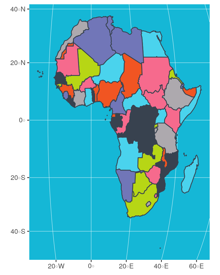

Tips: Do you need help for your SQL query ?

PostGIS allows you to make SQL queries with geomatics functions that you can also define before reading your dataset with {sf}. However, if you are not totally comfortable with SQL but you are a ninja with {dplyr}, then you will be fine. By using dplyr::show_query, you can get the SQL syntax of your {sf} operations. Let’s take an example.
With {sf}, union of countries by continent could be written as follows:

world_sf %>% 
 group_by(continent) %>% 
  summarise()

Indeed, the complete {sf} code would be:

world_sf %>% 
 group_by(continent) %>% 
  summarise(geometry = st_union(geometry))

Now, let us connect to the Postgres database with {dplyr}. When connected to a database with {dplyr}, queries are executed directly in SQL in the database, not in the computer memory.
Then use show_query to get the translation in SQL proposed by {dplyr}.
Note that with {dbplyr} (>1.4.0), instead of tbl, you can use a lazy_frame without real connection to the database to do your tests.

# Read with dplyr directly in database
world_tbl <- tbl(con, "ne_world")
# Create query
world_tbl %>% 
 group_by(continent) %>% 
  summarise(
   geometry = st_union(geometry)) %>% 
 show_query()

## <SQL>
## SELECT "continent", ST_UNION("geometry") AS "geometry"
## FROM "ne_world"
## GROUP BY "continent"

{dplyr} has not been tailored to translate spatial operations in SQL, but as you can see below, difference with the correct query is very small. Only the PostGIS function is not correctly written (ST_Union).

query <- paste(
  'SELECT "continent", ST_Union(geometry) AS "geometry"',
  'FROM "ne_world"',
  'GROUP BY "continent";'
)
union_sf <- st_read(con, query = query, quiet = TRUE)
# Plot (Choose your own palette)
union_sf %>% 
  st_transform(world_map_crs) %>%
  ggplot() +
  geom_sf(aes(fill = continent), colour = thinkr_cols("dark")) +
  scale_fill_thinkr_d(palette = "discrete2_long", guide = FALSE) +
  theme(panel.background = element_rect(fill = thinkr_cols("primary_light")))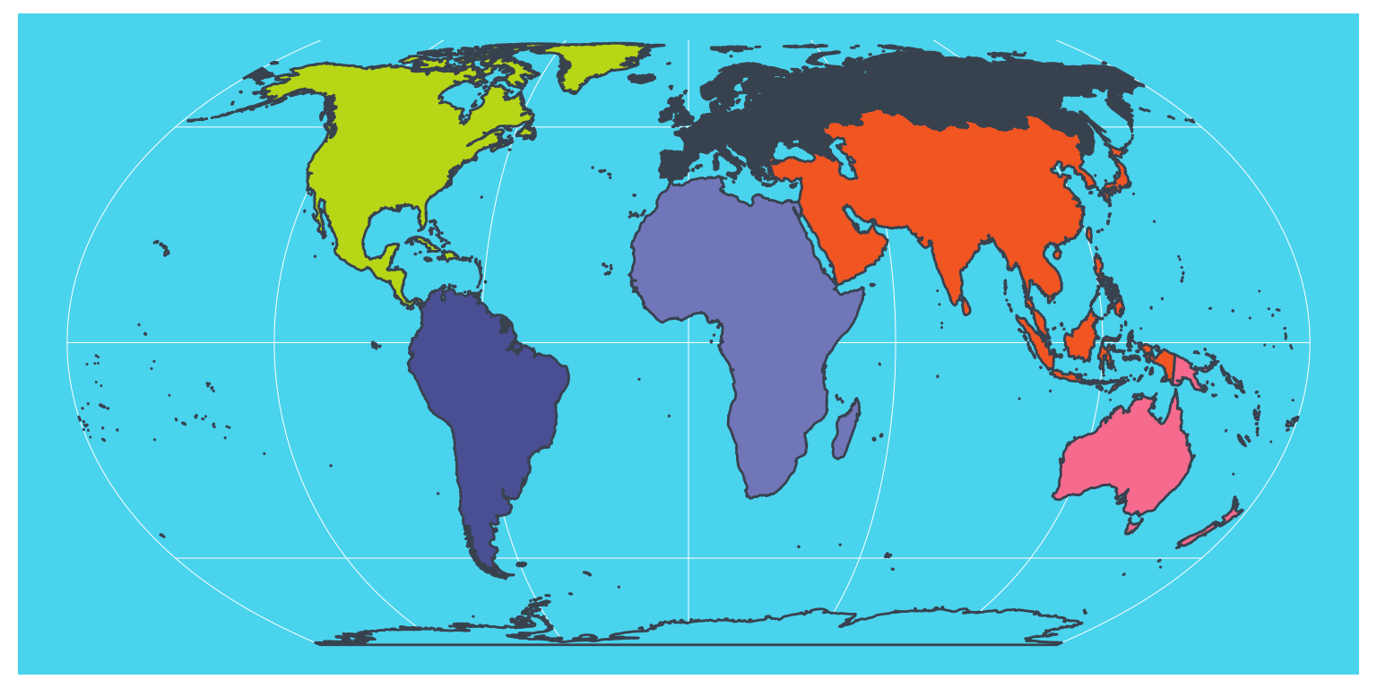

Be careful. You can not trust operations with {dplyr}/{dbplyr} on a spatial database because the ‘geometry’ column is not imported as spatial column with tbl() and you would loose it. However, you can use {dplyr} syntax to explore your dataset and all columns out of the spatial information. All operations will be realised inside the database, which assures not to overload the memory.

What about rasters ?

If you follow this blog, you know that I like rasters. Package {sf} is only dealing with spatial vector objects. It can not manage rasters in a PostGIS database. To do so, you can have a look at package {rpostgis} with functions pgGetRast() and pgWriteRast(). This package works with Rasters from package {raster}. You will need to connect using package {RPostgreSQL}, which does not have a Rstudio “connexion contract”. 

• Connect to the database with {RPostgreSQL}

library(rpostgis)
con_raster <- RPostgreSQL::dbConnect("PostgreSQL",
  host = "localhost", dbname = "postgres",
  user = "postgres", password = "mysecretpassword", port = 5432
)
# check if the database has PostGIS
pgPostGIS(con_raster)

## [1] TRUE

• Create an empty raster and save it in the database

# From documentation basic test
r <- raster::raster(
  nrows = 180, ncols = 360, xmn = -180, xmx = 180,
  ymn = -90, ymx = 90, vals = 1
)
# Write Raster in the database
pgWriteRast(con_raster,
  name = "test", raster = r, overwrite = TRUE
)

## [1] TRUE

• Read the raster from the database

r_read <- pgGetRast(con_raster, name = "test")
print(r_read)

## class       : RasterLayer 
## dimensions  : 180, 360, 64800  (nrow, ncol, ncell)
## resolution  : 1, 1  (x, y)
## extent      : -180, 180, -90, 90  (xmin, xmax, ymin, ymax)
## coord. ref. : +proj=longlat +datum=WGS84 +ellps=WGS84 +towgs84=0,0,0 
## data source : in memory
## names       : layer 
## values      : 1, 1  (min, max)

• Do not forget to close the database connection after your operations

# Disconnect database
RPostgreSQL::dbDisconnect(con_raster)

## [1] TRUE

Disconnect database and close Docker container

• Disconnect database connection made with {DBI}
• Stop and remove Docker container if wanted

# Disconnect database
DBI::dbDisconnect(con)
# Stop Docker container
system2("docker", "stop some-postgis")
system2("docker", "rm --force some-postgis")
# Verify docker
system2("docker", "ps -a")

To go further

• ThinkR provides expertise for your infrastructure installation around R and Rstudio products
• ThinkR teaches how to deal with spatial data in R. This includes PostGIS databases.
• Documentation on PostGIS
• Package {sf} development repository
• Introduction to spatial data manipulation with {sf} by Sébastien Rochette (me)
• Geocomputation in R by Robin Lovelace et al.
• Introduction to Docker by Colin Fay
• Introduction to R, databases and Docker by John David Smith et al.

Packages used in this blogpost

# remotes::install_github("ThinkR-open/attachment")
sort(attachment::att_from_rmd("2019-04-27_postgis.Rmd"))

##  [1] "attachment"     "DBI"            "dbplyr"         "dplyr"          "ggplot2"        "knitr"          "raster"        
##  [8] "rnaturalearth"  "rpostgis"       "RPostgres"      "RPostgreSQL"    "sf"             "sqlpetr"        "thinkridentity"