Can mapping tools be diverted to other uses? Of course ! See how we play with leaflet and leafgl to quickly render a giant waffle made of millions of polygons.
Spatial tools are not only for spatial data
Table of Contents
At SatRday in Paris, I presented a talk entitled “Everything but maps with spatial tools”.
The aim is to show that there exists powerful tools in some fields that can be applied to other fields. You just have to open your mind a little bit. Personally, I like playing with maps and spatial data. In fact, I see rasters everywhere…

In this blog post, I present a small part of my talk. It seems that whatt has left its mark on people’s minds is the waffle story… So, this is the first one I will share with you !
Waffles are electronic components
At ThinkR, we develop and deploy Shiny applications. In this case, it is for a client working with electronic components. I can not say more about this work. This is why I used this analogy with waffles.
Open your mind I said ! Use your imagination.
Imagine the world largest waffle. A waffle with millions of cells.
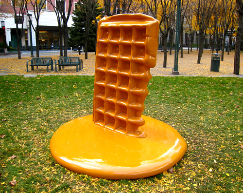 |
| Brooklyn, Martha Friedman Waffle |
We’re going to add some chocolate on it. However, we are not really good at it and it is not possible to put the same quantity of chocolate in each cell.
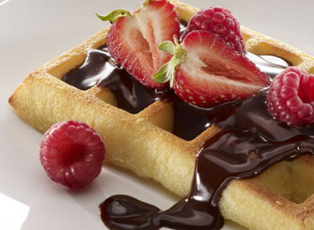
For each cell, we know the coordinates of its center. We know the quantity of chocolate. In this job, we want to be able to:
- Explore each cell if needed
- Zoom in/zoom out over this millions of cells
- Show this waffle in a Shiny application
- Switch from one waffle to another as smoothly and quickly as possible
A raster is a multipolygons structure
A package that recently appeared among spatial tools within R is {leafgl}. This is a Github only R package available here: https://github.com/r-spatial/leafgl. It allows quick rendering of millions of points using leaflet.
Waffles were the perfect opportunity to test this package !
A waffle is a regular grid. This may be seen as a raster. However, {leafgl} only works with vector objects. Of course, {leaflet} can print rasters, but this was not quick enough for us. Not always, but sometimes speed matters…
So again, open your mind and try to see a spatial vector when looking at a raster.
library(raster)
library(rasterVis)
library(waffler)
library(cowplot)
# Build a raster
mat <- matrix(c(1, 0, 0, 1), ncol = 2)
r <- raster(mat)
plot(r)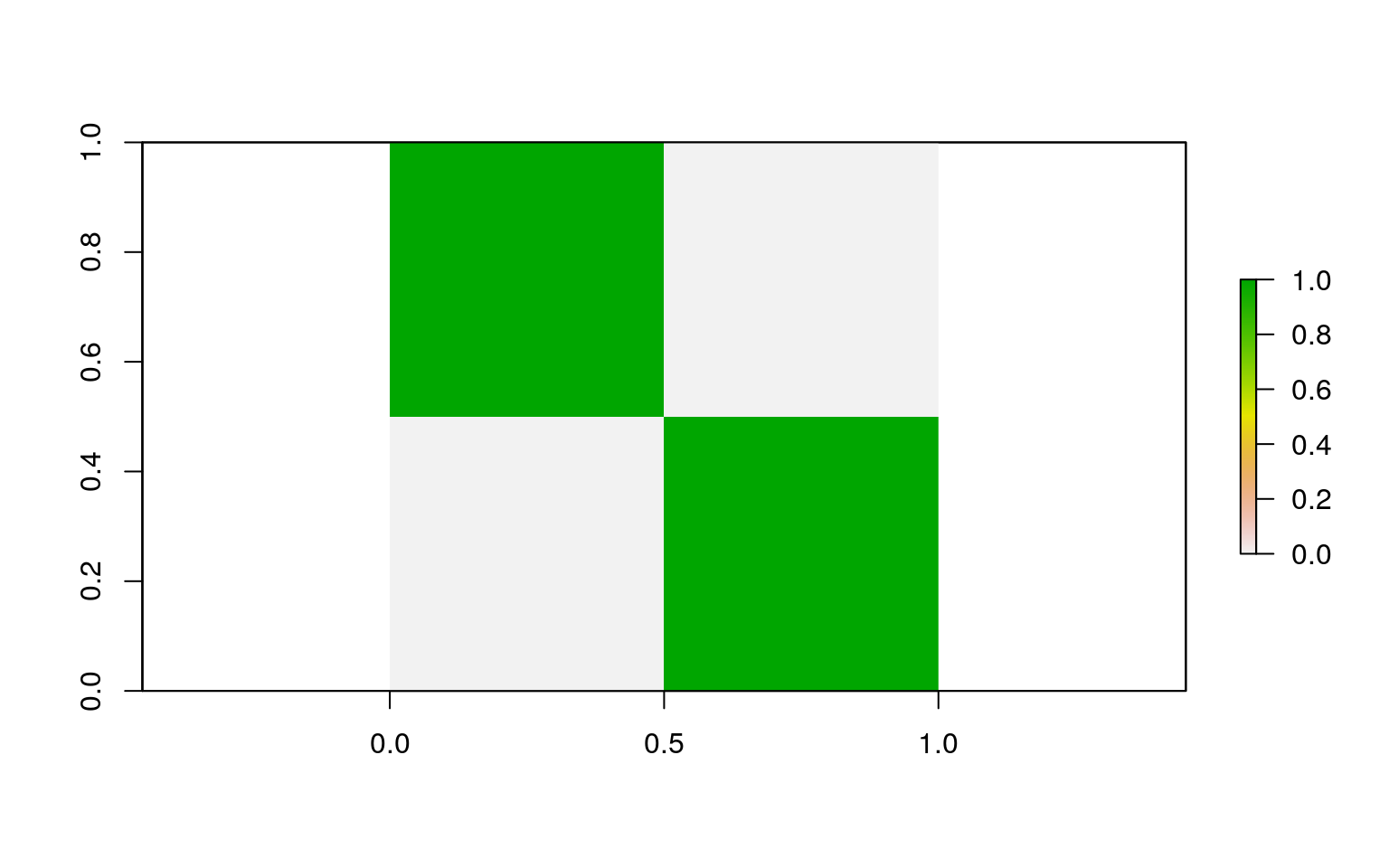
# Get centers
r_df <- data.frame(coordinates(r), values = values(r))
# Transform as polygons
r_waffle <- wafflerize(r_df)
g1 <- gplot(r) +
  geom_raster(aes(fill = value)) +
  guides(fill = FALSE) +
  ggtitle("Original raster")
g2 <- ggplot(r_waffle) +
  geom_sf(aes(colour = LETTERS[1:nrow(r_waffle)]), size = 2) +
  guides(colour = FALSE) +
  ggtitle("Raster as polygon")
plot_grid(plotlist = list(g1, g2))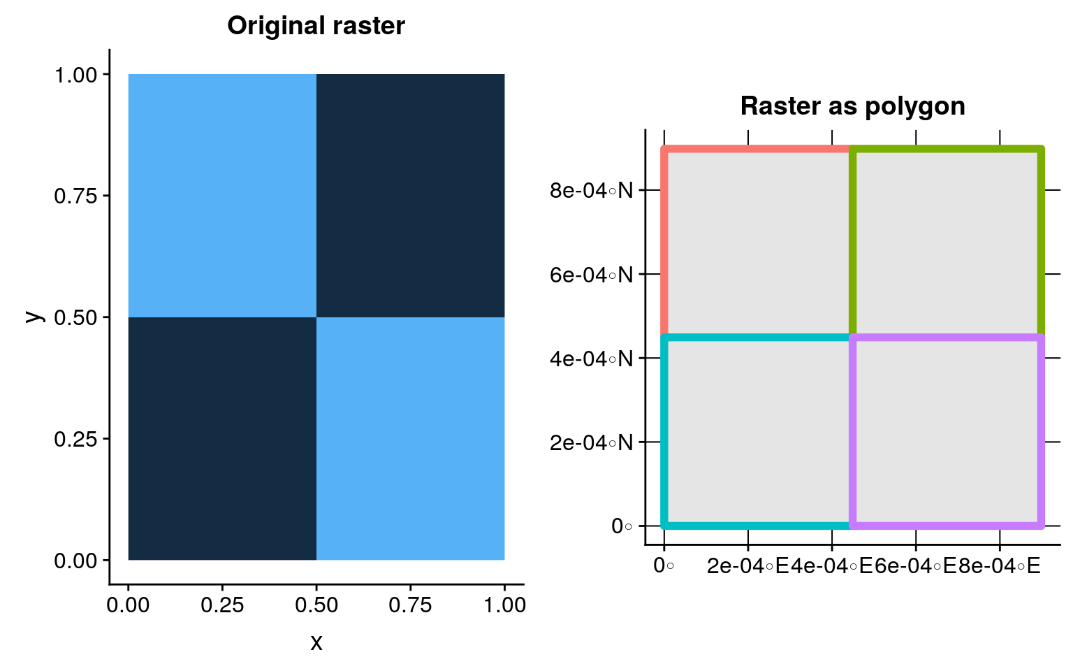
Do you see rasters as polygons now ?
So we’re going to play with a bigger waffle! We can, so why would we deprive ourselves of it?
Plot an heart-shaped waffle
A rectangle is boring, let’s build a heart shaped waffle with {sf}. The heart is a polygon from which we can extract a regular set of point using st_sample. This set of point symbolizes the center of each waffle cell. Then we can generate more or less chocolate in each cell.
The trick is to use spatial tools on non-spatial data. The heart we draw is not to be placed on a real position on Earth. > Indeed, I am currently writing this blog post in the train (#OnTheTrainAgain as says Colin), thus the heart drawn has no fixed position. Even if I am on Earth, my train is not following a heart shaped path. Well, you understand the idea…
Hence, to be able to play with this polygon, it is better to assign it a projection. Let’s add a Lambert93 projection (EPSG: 2154), because I am in France !
library(sf)
# Construct heart (code from @dmarcelinobr)
xhrt <- function(t) 16 * sin(t)^3
yhrt <- function(t) 13 * cos(t) - 5 * cos(2 * t) - 2 * cos(3 * t) - cos(4 * t)
# create heart as polygon
heart_sf <- tibble(t = seq(0, 2 * pi, by = .1)) %>%
  mutate(y = yhrt(t),
         x = xhrt(t)) %>%
  bind_rows(., head(., 1)) %>%
  dplyr::select(x, y) %>%
  as.matrix() %>%
  list() %>% st_polygon() %>%
  st_sfc(crs = 2154)
g1 <- ggplot(heart_sf) +
  geom_sf(fill = "#cb181d") +
  coord_sf(crs = 2154, datum = 2154) +
  ggtitle("Heart sf polygon")
# create grid
heart_grid <- st_sample(heart_sf, size = 500, type = "regular") %>%
  cbind(as.data.frame(st_coordinates(.))) %>%
  rename(x = X, y = Y) %>%
  st_sf() %>%
  mutate(z = cos(2*x) - cos(x) + sin(y),
         z_text = paste("Info: ", round(z)))
g2 <- ggplot(heart_grid) +
  geom_sf(colour = "#cb181d") +
  coord_sf(crs = 2154, datum = 2154) +
  ggtitle("Heart as regular point grid")
g3 <- ggplot(heart_grid) +
  geom_sf(aes(colour = z), size = 2) +
  scale_colour_distiller(palette = "YlOrBr", type = "seq", direction = 1) +
  theme(panel.background = element_rect(fill = "#000000")) +
  coord_sf(crs = 2154, datum = 2154) +
  guides(colour = FALSE) +
  ggtitle("Chocolate quantity for each point")
cowplot::plot_grid(g1, g2, g3, ncol = 3)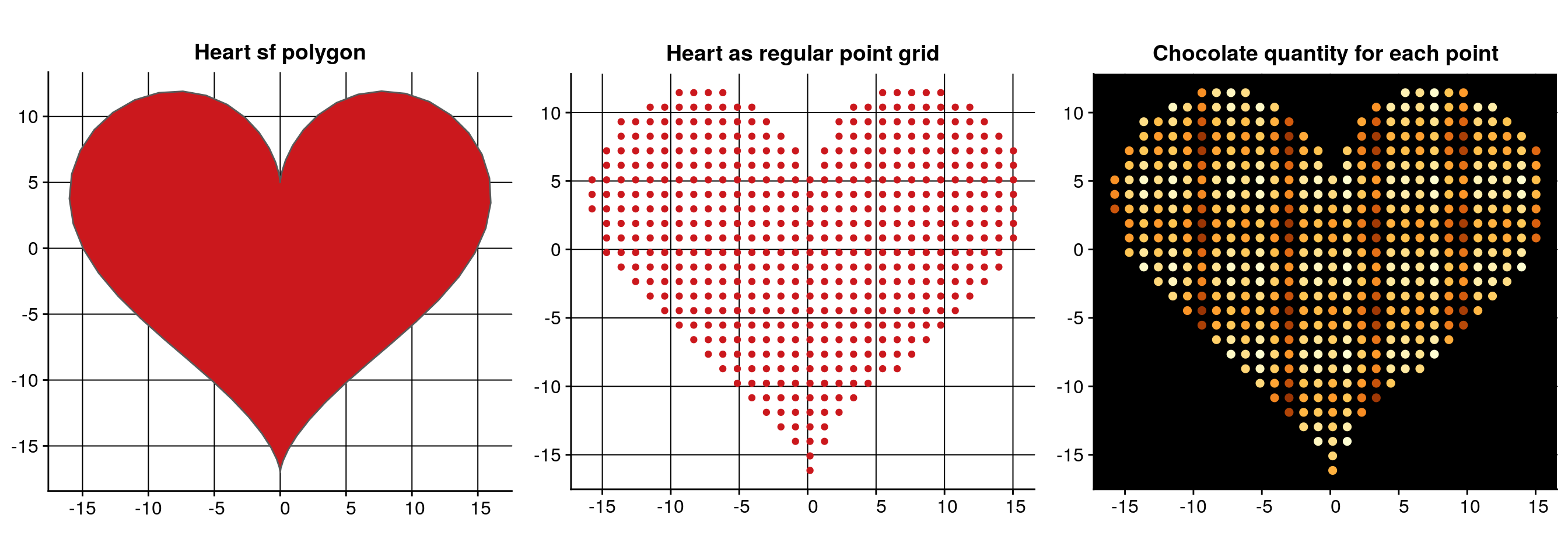
The projection chosen is however a problem. {leaflet} requires spatial objects with non-projected geographic coordinates (EPSG: 4326). Why didn’t I assign directly coordinates in degrees, then ? Because {leaflet} produces a map in Mercator projection (EPSG: 3857), and I do not want my heart to be deformed by the change in projection. Why didn’t I assign a Mercator projection then ? Because I like maps and I dislike Mercator as it gives a really bad representation of distances and surfaces of our World. But this is another problem… In our case, I will indeed have to create my polygon grid with a Mercator projection, transform it as geographic coordinates, so that my heart is not in a bad mood on the final map.
To transform a regular set of points into a polygon grid ready for leaflet while integrating deformation, I created package {waffler}, available on Github only (https://github.com/ThinkR-open/waffler). Use devtools::install_github("ThinkR-open/waffler") to try it.
We’ll use function wafflerize. The fact parameter is here to magnify the size of the heart. If we keep a resolution of 1 for a 500x500 square waffle, this will be too small to appear with distinguishable geographical coordinates.
# Generate a grid polygon from points
heart_polygon <- wafflerize(heart_grid, fact = 1000000)
g1 <- ggplot(heart_polygon) +
  geom_sf(aes(fill = z), colour = "blue", size = 0.5) +
  scale_fill_distiller(palette = "YlOrBr", type = "seq", direction = 1) +
  theme(panel.background = element_rect(fill = "#000000")) +
  coord_sf(crs = 4326, datum = 4326) +
  guides(fill = FALSE) +
  ggtitle("Chocolate quantity (geographical coordinates = data)")
g2 <- ggplot(heart_polygon) +
  geom_sf(aes(fill = z), colour = "blue", size = 0.5) +
  scale_fill_distiller(palette = "YlOrBr", type = "seq", direction = 1) +
  theme(panel.background = element_rect(fill = "#000000")) +
  coord_sf(crs = 3857, datum = 3857) +
  guides(fill = FALSE) +
  ggtitle("Chocolate quantity (Mercator projection = leaflet)")
plot_grid(plotlist = list(g1, g2), ncol = 2)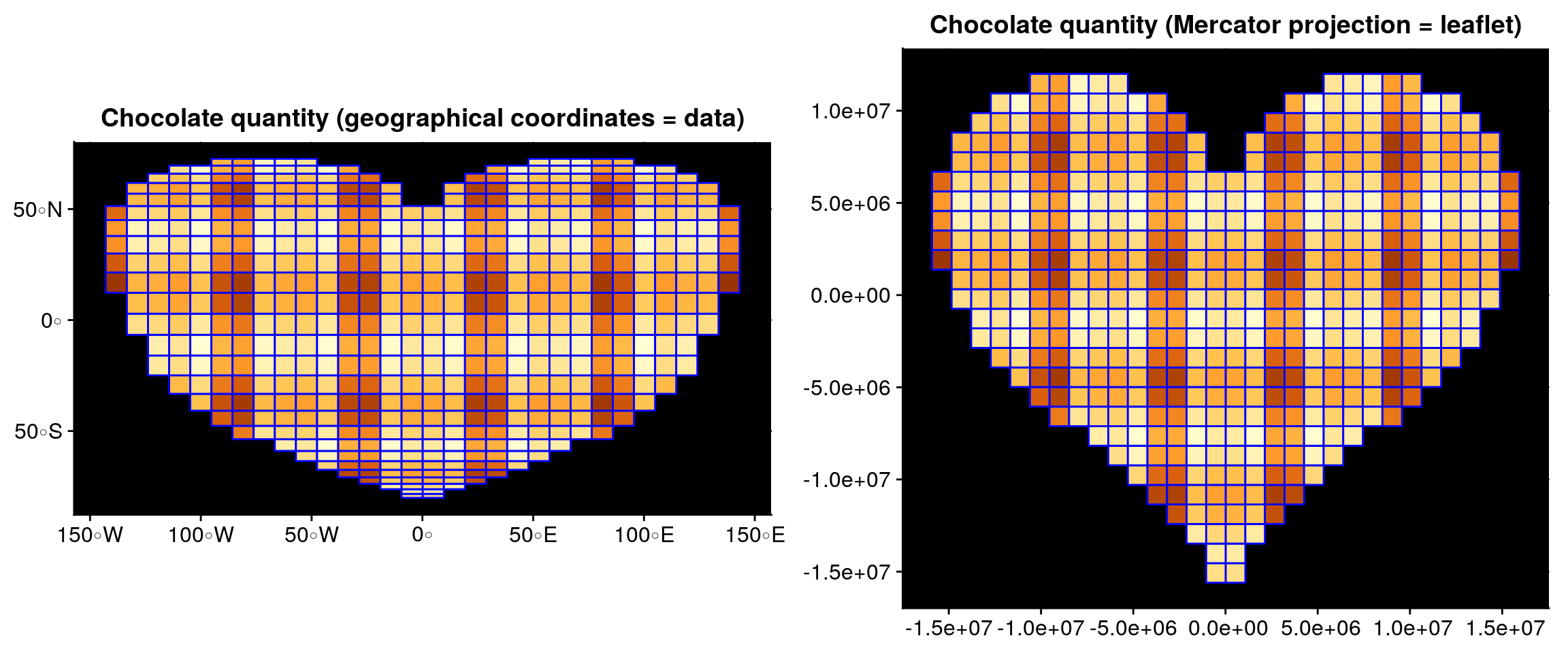
Plot a big interactive waffle
We’re almost there! Remember that our objective was to build an interactive waffle.
For the demonstration, we build a bigger heart with 50000 points. Let’s plot it with {leafgl}.
library(leaflet)
library(leafgl)
# Bigger heart
heart_grid <- st_sample(heart_sf, size = 50000, type = "regular") %>%
  cbind(as.data.frame(st_coordinates(.))) %>%
  rename(x = X, y = Y) %>%
  st_sf() %>%
  mutate(z = cos(2*x) - cos(x) + sin(y),
         z_text = as.character(round(z, digits = 1)))
# Generate a grid polygon from points
heart_polygon2 <- wafflerize(heart_grid, fact = 100)
# Define colors for `addGlPolygons`
cols <- brewer_pal(palette = "YlOrBr", type = "seq")(7)
colours <- gradient_n_pal(cols)(rescale(heart_polygon2$z))
colours_rgb <- (t(col2rgb(colours, alpha = FALSE))/255) %>% as.data.frame()
# Render as leaflet
m <- leaflet() %>%
  # The popup is currently not working anymore with {leafgl}.
  # I cheat a little and take the previous version waiting for a patch...
    leaflet.glify::addGlifyPolygons(data = heart_polygon2, # addGlPolygons(
                color = colours_rgb,
                popup = "z_text",
                opacity = 1) %>%
  setView(lng = mean(st_bbox(heart_polygon2)[c(1,3)]),
          lat = mean(st_bbox(heart_polygon2)[c(2,4)]), zoom = 15)
You can now navigate inside this polygon-raster object. Click on the cells to know the quantity of chocolate…
Next time you’ll see waffles in the wild, you may think about me…
